In many radiation detection projects, the physics works.

The detector responds.
The spectrum is visible.
The peaks are where they should be.

And yet, the system fails when moved outside the laboratory.

Why?

Because laboratory instrumentation and deployable systems are two fundamentally different engineering problems.

The Illusion of “Working”

A laboratory setup typically consists of:

• a detector (PMT or SiPM-based),
• a commercial digitizer,
• external power supplies,
• a PC running analysis software,
• controlled temperature and stable background conditions.

In this configuration, the system appears stable and reliable.

But this stability is often conditional.

Remove the PC.
Increase the count rate.
Change the temperature.
Add mobility.

The system behaviour changes.

Where the Gap Appears

The transition from laboratory setup to field-oriented system usually exposes several bottlenecks:

1. Spectral Drift

In high count-rate or temperature-varying environments, peak positions begin to move.

Without active stabilization or real-time correction, calibration becomes unstable.

2. Dead Time and Pile-Up

Laboratory digitizers are often optimized for flexibility, not for sustained high CPS operation.

Under dynamic conditions, dead time increases and pile-up distorts spectral shape.

3. External Processing Dependency

Many systems rely on a PC for:

• pulse processing,
• time correlation,
• spectral separation,
• data filtering.

This architecture is unsuitable for autonomous or embedded deployment.

4. Integration Complexity

Combining:

• HV supplies,
• front-end electronics,
• digitizers,
• synchronization logic,
• software control

often results in a fragile ecosystem of loosely coupled components.

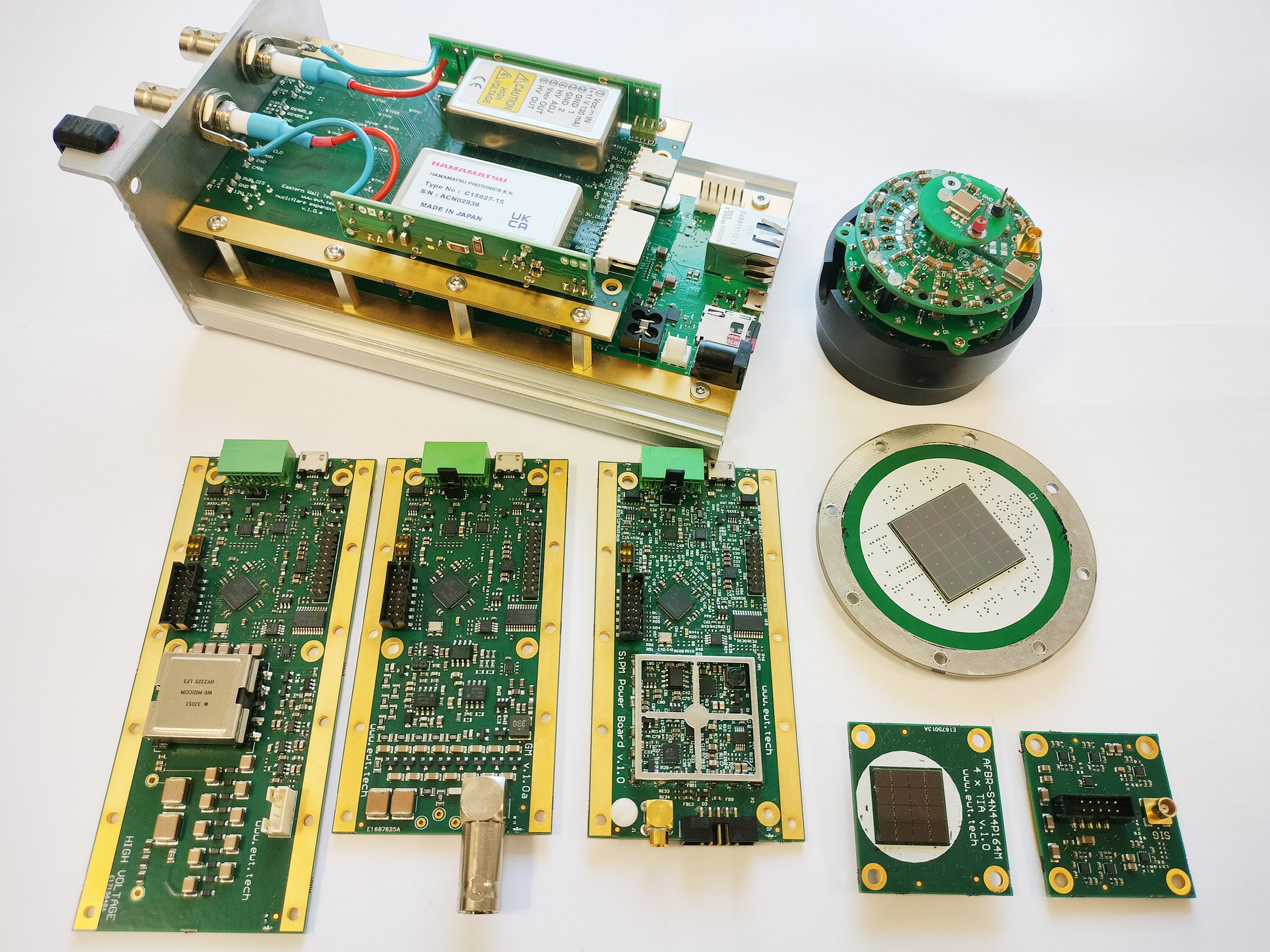
What Changes in a Standalone Architecture?

A deployable radiation measurement system requires:

• embedded real-time digital pulse processing,
• minimal dead time at high count rates,
• stable baseline behaviour under dynamic conditions,
• integrated high-voltage control,
• deterministic timing and synchronization,
• autonomous spectral analysis.

In other words:
the entire measurement chain must be engineered as one system, not assembled from loosely connected laboratory modules.

The Practical Reality

In most projects, the limiting factor is not detector physics.

It is the time and engineering effort required to transform a working laboratory setup into a stable, application-ready device.

This is where modular, application-oriented measurement electronics become critical.

Not because they are “more advanced”, but because they are designed from the beginning for:

• stability under non-ideal conditions,
• high sustained event rates,
• embedded operation,
• integration into larger systems.

What This Blog Will Show

Future posts will document practical aspects of this transition:

• how to manage baseline stability at high CPS,
• how to design time-correlated acquisition systems,
• how to move from PC-based analysis to embedded processing,
• how to simplify system integration using modular building blocks.

The goal is not to criticize laboratory instrumentation.

It is to clarify that laboratory tools and field systems serve different purposes — and require different design decisions.